Simplifying CUDA kernels with Triton: A Pythonic Approach to GPU Programming

Writing custom CUDA kernels for whatever reasons had always looked like a daunting task. This is where OpenAI’s triton comes in handy. With its pythonic and torch like syntax now its a bit more approachable. So lets dive in and see what triton has to offer.

Understanding GPU Memory Hierarchy

Before that lets have a quick introduction about how GPU memory works. I want to keep this short. I will leave the resources for extra reading here. But long story short there are two main kinds of memory in GPUs.

1. GPU DRAM (also known as High Bandwidth Memory, HBM): The typical memory we refer to when we say the GPU has a memory of 16GB or 80 GB etc. Think of it like memory in your backyard warehouse. This is slower but inexpensive to make compared to SRAM. For A100 for example the memory bandwidth for this kind of memory, is ~2TB/s
2. GPU SRAM (L1/L2 Caches): This is much smaller in size usually in KBs and MBs which is more local to the chip (within the die) , hence much faster to access, at the same time more expensive to make. This is sort of like the working memory of the chip. For A100 the L1 Cache size is 192KB per Streaming Multiprocessor (SM)(think of it like a bunch of cores lined up together) and L2 Cache Size is 40MB (think of it as memory inside the house)
   For A100s again:
   L1 Cache Bandwidth: ~100–200 TB/s theoretical bandwidth
   L2 Cache Bandwidth: ~4–7 TB/s theoretical bandwidth

L1 Caches are like memory you have available on the table you are working on, L2 is more like somewhere in the room where you are working on and DRAM is probably in your backyard warehouse. Hence the difference in speed. Now you get the idea of where the speed lies. The key thing here is accessing memory from within these caches is much faster, and the SM has to wait a lot less shorter if data is available within these. These modern cores can perform multiple 100s of cycles during DRAM access times and that goes down to only 10s of cycles if the data is in the L1 Cache. So this is the cost of data movement!

Triton Basics: Thread Launching and Block Processing

Okay lets get back. Imagine you have to add/multiply 2 vectors of size 50k. I know 50k is just arbitrary and I chose it to make a point, clearly. With the 192KB of memory highway available to you, you want to make the best use of it. If we are talking about FP32 numbers within these vectors then the vector is already well beyond what can be stored within these tiny units of memory.

And you have 2 of these and still need that much space to store the outputs. So in triton or CUDA in general the way this is dealt with is by using block sizes. You can still get the same output if each SM is only looking at a partition of the data of size Block Size

Practical Example: Vector Addition in Triton

Now for example in our 60k vector, if we divide it into a non-overlapping blocks of size 8k each, the last block will only have 4k numbers. If we always assume we will have block size elements, we will need a mechanism to tell CUDA or triton that just look at the 4k in this last block ignore the other half. This is where masks come in. Now I will put this all together into a logical flow:

Lets see how to do this. I will first start with how we launch these threads in the first place. I will use the snippet from official triton docs here with some changes to make it a bit more readable

import triton
import triton.language as tl

@triton.jit
def add_kernel(x_ptr,
               y_ptr,
               output_ptr,
               n_elements,
               BLOCK_SIZE: tl.constexpr):
  # We will shortly get to this part
  pass

def add(x: torch.Tensor, y: torch.Tensor, BLOCK_SIZE: int = 1024):
  # In practice we use 2's powers wherever possible, some perf advantage
  # We need to preallocate the output.
  output = torch.empty_like(x)
  assert x.device == DEVICE and y.device == DEVICE and output.device == DEVICE
  n_elements = output.numel()
  # The SPMD launch grid denotes the number of kernel instances that run in parallel.
  # It is analogous to CUDA launch grids. It can be either Tuple[int], or Callable(metaparameters) -> Tuple[int].
  # In this case, we use a 1D grid where the size is the number of blocks:
  # This is just a ceiling division i.e a//b + 1
  grid = (triton.cdiv(n_elements, BLOCK_SIZE), )
  # NOTE:
  #  - Each torch.tensor object is implicitly converted into a pointer to its first element.
  #  - `triton.jit`'ed functions can be indexed with a launch grid to obtain a callable GPU kernel.
  #  - Don't forget to pass meta-parameters as keywords arguments.
  add_kernel[grid](x, y, output, n_elements, BLOCK_SIZE)
  # This would update the output in-place
  return output

So here we launched a 1-D grid of threads/processes which is supposed to handle non-overlapping parts of the data and process and dump data independently into the output. Like the note says a key thing to note here is that the x_ptr or y_ptr that triton sees is sort of like an address to the very first element of the tensor (array in this case). Okay now lets see how to do this exactly:

@triton.jit # This just compiles the code to GPU language so to speak
def add_kernel(x_ptr,
               y_ptr,
               output_ptr,
               n_elements,
               BLOCK_SIZE: tl.constexpr):
  
    # This is shared across many processes in the launch grid we set
    pid = tl.program_id(axis=0)  # This tells us the index of the thread
    # This would be like 0, 1, 2, .... upto the number of threads in that dim

    # The first thread should look at the data from [0:1024]
    # The second should look at the data from [1024: 2048] and so on
    block_start = pid * BLOCK_SIZE
    offsets = block_start + tl.arange(0, BLOCK_SIZE)
    # Create a mask to guard memory operations against out-of-bounds accesses.
    # Think of the last thread in our toy example. last 4k in our offset is
    # out of bounds for our original data
    mask = offsets < n_elements
    # Load x and y from DRAM, masking out any extra elements in case the input is not a
    # multiple of the block size.
    x = tl.load(x_ptr + offsets, mask=mask) # These are loaded onto the SRAM
    y = tl.load(y_ptr + offsets, mask=mask) # These are loaded onto the SRAM
    output = x + y
    # Write x + y back to DRAM.
    tl.store(output_ptr + offsets, output, mask=mask)

To summarize, this is like any parallel processing logic. We just need to decide on an access pattern so to speak, which processes chunks of data without any race-conditions like 2 processes simultaneously trying to access the same data pointer and the like.

Advanced Implementation: Matrix Multiplication

Now that’s out of the way lets look at a bit more complicated example of matrix multiplication. Now bear in mind the kernel that you are about to read is not the most optimal implementation of matrix multiplication. This is just so that we can get our hands dirty and also not everything you do has to be efficient. It just has to work, and you would have learned a lot in the process. I am just going to leave the kernel here for you to get a hang of it.

@triton.jit
def simple_mm(a, b, o, k, n,
              K_BLOCK_SIZE: tl.constexpr = 64,
              ) -> None:
    # a -> Matrix of size M x K and b -> Matrix of size K x N
    # K is the common inner dimension
    num_blocks = k//K_BLOCK_SIZE + 1
    row_id = tl.program_id(0)
    col_id = tl.program_id(1)

    # Lets pick one column and one row and do a dot product
    # Like the 1-D example we dont want to look at the entire row/column
    # We are making use of the fact that each row/column will be of the size
    # 'k' which is the inner common dimension of these matrices
    # But this will only be a part of the dot product so we have to keep track of many to cover the entire column or row.
    
    # What we are going to do is to access block size elements from the column
    # and the row and compute the dot product and keep adding to a value till
    # we run out of numbers
    value = 0.
    for k_id in range(num_blocks):
        row_start = row_id * k + k_id * K_BLOCK_SIZE
        row_offsets = tl.arange(0, K_BLOCK_SIZE) + row_start
        # The masks are a little more trickier as we cant just see if its
        # less than 'k'. We need to account for the row we are in
        row_masks = row_offsets < (row_id + 1) * k
        row = tl.load(a + row_offsets, mask=row_masks) # Load this into the GPU SRAM

        col_start = (K_BLOCK_SIZE * k_id)
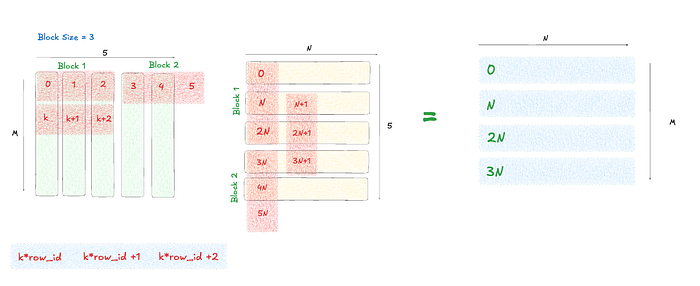
        col_offsets = n * (tl.arange(0, K_BLOCK_SIZE) + col_start) + col_id # 0, n, 2n || 3n, 4n, 5n for a block size of 3 for eg
        col_masks = col_offsets/n < k
        col = tl.load(b + col_offsets, mask=col_masks)
        value += tl.sum(row * col)
    
    output_offset = row_id * n + col_id
    tl.store(o + output_offset, value)

I am also leaving a rough sketch of how these access patterns came about. The numbers you see below are the indexes of those positions, if we were to flatten this matrix out. This would in turn be our memory offsets/differences in the ptr from the first element in the matrix. It goes row wise first.

Resources for Further Learning

Nexts steps would be to try and implement custom kernels for all sorts of things, like a cross-entropy loss, or a softmax etc. Hope you get the idea. I tried to keep it short. If you want to learn more I am leaving you with a few good resources to have a look at:

1. An advanced implementation of a custom Cross Entropy Loss kernel from Unsloth
2. Official Triton Documentation
3. and Claude ofc. Makes the learning a whole lot easier!

As ML models continue to grow, what role do you see for Python-based GPU programming languages versus traditional CUDA? Is Triton filling a temporary gap or establishing a new paradigm?